Home page of EDISP
(English) DIgital Signal Processing course
winter 2008/9

Schedule

Short info: labs will be on Mondays, 8-12 , in two subgroups of not more than 12 students. We will have to multiplex in odd/even week with EMISY.
For the introductory lab (lab0) we met on 20 Oct, 9:15 room 022.
Next lab (lab1) will be

• 27.10.2007 (8:15-12) for N subgroup,
• 03.11.2007 (8:15-12) for P subgroup

As for now, we assume that "N" subgroup will have labs on weeks marked as "N" in the official elka calendar (and "P" on "P" weeks).

Books

A. V. Oppenheim, R. W. Schafer, Discrete-Time Signal Processing, Prentice-Hall 1989 (or II ed, 1999; also acceptable previous editions entitled Digital Signal Processing).

A free textbook covering some of the subjects can be found here: http://www.dspguide.com/pdfbook.htm
The book is slightly superficial, but it can be valuable - at least as a quick reference. Additional books available in Poland:

• R.G. Lyons, Wprowadzenie do cyfrowego przetwarzania sygnałów (WKiŁ 1999)
• Craig Marven, Gilian Ewers, Zarys cyfrowego przetwarzania sygnałów, WKiŁ 1999 (simple, slightly too easy) [en: A simple approach to digital signal processing, Wiley & Sons, 1996]
• Tomasz P. Zieliński, Od teorii do cyfrowego przetwarzania sygnałów, WKiŁ 2002 (and next edition with slightly modified title)

Please remember:

• there are notation differences between lecture and "dspguide"
• The official book is Oppenheim & Schafer (though notation is sometimes different too)
• no book is obligatory in these circumstances

Probably the best choice is to buy O&S. It'll serve you for years, if you are interested in DSP. And it contains a lot of PROBLEMS to solve and learn!

Or you may prefer to buy/borrow a laboratory scriptbook, which is in Polish language (Cyfrowe Przetwarzanie Sygnałów, red. A Wojtkiewicz, Wydawnictwa PW).
 

Lecture slides

Lecture number = week number in schedule.

• Lecture 1 slides: newlect1.pdf but please don't read the schedule there - use the schedule.pdf
• Lecture 2 slides: newlect2.pdf
  Convolution example: conv_exampl.jpg
• Lecture 3 slides: newlect3.pdf
• Lecture 4 slides newlect4.pdf
  Homework will be given this day!
• Lecture 5:
  Windowing for DFT, DFT applications slides: newlect5.pdf
  Instantaneous spectrum: newlect6.pdf
  
• Lecture 6: (11.11)Independence Day - holiday!
  
• Lecture 7:(18.11)
  Homework (hand-written on paper, worth up to 2 points) is due at the BEGINNING of the lecture.
  Review (for the test; based also on your homework errors)
  Lecture "Linear difference equations" - last 3 slides from newlect2.pdf
  and Z-transform newlect7.pdf
  
• Lecture 8(25.11): (test I -> postponed to 2.12)
  Filters part I:newlect8.pdf
  Review after homework / before test I.
• Lecture 9(2.12): (++1) hour test I , 10pts worth: bring YOUR OWN notes (handwritten on paper or on printed lecture slides). No books, no photocopies of other person notes. Example test:test1_078a.pdf
  
• Lecture 10(9.12):
  last slides of Filters part I
  Filters part II:newlect9.pdf
  Filters part IIInewlect10.pdf (and maybe more...)
• Lecture 11: Digital signal processors: lect12_dsp.pdf(and OHP foils to be seen at the lecture)
  Homework:(homew2.pdf) given today
• Lecture 12: Random DT signals lect9.pdf
• Lecture 13/14: Merry Christmas and Happy New Year
• Lecture 15: 2D signal processing lect13.pdf
  Homework due today
• Lecture 16: test II ( example test here)
• Lecture 17: advanced techniques including signal processing for data compression
• Lecture 18: Exam 0: pen, pencil, calculator and your own notes plus lecture slides. Copies of solutions for homeworks/tests/exams are NOT allowed.
  The exam covers ALL the course matter. There are "Problems" (longer) and "Questions" (shorter), for total of 90 minutes.
  Exam 0 is a "bonus" - if you fail you are still entitled to take Ex1 and Ex2 and no "bad" record remains.

Examples of final tests (historical)

One test. Another test.

There is no guarantee that the current test be identical ;-). It will be similar (the lecture was similar), but I might also put more focus on different subjects. The only base is the lecture content (live one, not only the published slides ....).

The main rule: exam covers the whole course content (sampled), including the T1(H1)+T2(H2) area and also the lectures after the H2.

Lab info: example lab exercises

Disclaimer:

Openly speaking, they are exercise sets current at the time of posting. I reserve the right to make some important modifications before the actual lab, to give different sets to different groups etc. (and I usually DO review the text before giving it....).

• Lab 0: Introduction, Matlab
• Lab 1: Signals, systems, frequency
  • Simple MATLAB usage: make a vector, plot x - y plot with proper data on axes, make a simple m-function.
  • DT signal as a sampled CT signal: plot sample values of a sin() with a frequency of 1 kHz, sampled with 10 kHz (etc). Put x-axis values as sample index, CT instant, ....
  • Normalized frequency concept (e.g. What is the θ value in the above example?)
  Lab exercises: lab0a.pdf
• Lab 2: Spectral analysis (+ continuation of lab1)
  • Impulse response of a system; initial conditions etc.
  • DFT properties, effect of limited observation time (windowing)
  • Spectrum of a rectangular impulse
  Lab exercises: lab2plus1cd.pdf
• Lab 3: Instantaneous spectrum Lab exercises: lab03.pdf
• Lab 4: Filter design Lab exercises: lab4.pdf
• Lab 5: we don't do it (I'm just using old numbering scheme with 7 labs....)
• Lab 6: Signal processors Lab exercises: lab6.pdf
• Lab 7: Image processing Lab exercises: lab7.pdf

Homework solutions

Test2 solutions

Exam 0 solutions

Past things archive (Attic)

1. In both cases the signal was sampled correctly (f_s>2f)
   1. To calculate N₀ it was enough to count no. of samples in period (or divide f_s over f). Answer was 10(A) or 6(B). For N₀ samples in period, θ₀ was equal to 2π/N₀.
   2. K-size DFT will have K discrete samples over <-π, +π) (we include -π, and exclude +π , but due to periodicity of spectrum it is only a convention)
      for a cosine, only two samples are non-zero: at k such that θ_k=±θ_signal. Form the definition of θ_k you will see that this is for k=±4 (this is the result of taking K=4N₀).
   3. You may label frequency axis with k=-K/2,....-1,0,1,...K/2 or with its periodic equivalent K-K/2,....K-1,0,1,...K/2
      to label with θ just use the expression for θ_k.
2. 1. H(z)=Y(z)/X(z) is easily obtainable from the time equation. It was
      0.2(1+z^-1)/(1-0.8z^-1) [A]
      -0.2(1-z^-1)/(1+0.8z^-1) [B]
   2. Zeros are roots of numerator: -1 [A] or +1 [B]
      Poles are roots of denominator: +0.8 [A] or -0.8 [B]. They are inside unit circle, so the system is stable (but I didn't ask...)
   3. Example graph: 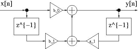- please find a_0, b_0, b_1 by yourselves. If you are smart, you may save one multiplication by 0.2 (this is left as exercise to you).
   4. For x(n)= shifted delta, (a limited energy signal) you may take the impulse response and shift it appropriately. To find h(n) it is easiest to split H(z) into two fractions: (shown for [A], for [B] change some signs)
      0.2(1/(1-0.8z^-1)+z^-1/(1-0.8z^-1))
      and lookup the inv.Z of 1/(1-0.8z^-1) in the table. The final result is a sum of two identical exponentials shifted by 1 in time. Then, you shift h(n) to proper position....
   5. For x(n) = 1-(-1)ⁿ (a periodic signal) we see a DC component and a periodic component exp(jπn) with frequency of π. We find numerical values of H(0)=(2 or 0) and H(π)= (0 or -2) by substituting exp(0) and exp(π) for z, and finally
      y(n)=H(0)-H(π)·(-1)ⁿ
3. The response was symmetrical around its midpoint (n= 2 or 4). Thus, it was a repsonse of a zero-phase filter delayed by 2 or 4.
   1. phase is linear φ=-(2 or 4)θ
      delay is constant and equal to (2 or 4)
   2. The response of filter is a rectangle modulated by exp(jπn). Thus, the characteristics is a sin(θL/2)/sin(θ), shifted to π. You may find the mainlobe width, you may plot exactly zeros of A(θ) etc.
4. Time resolution is proportional to time duration of window, frequency resolution - to mainlobe width (which is prop. to 1/K ....).
   Rectangular window has narrowest mainlobe possible, but high sidelobes; so it is good for resolving signals close in frequency, but without large difference in amplitudes.
   Any other window will have wider mainlobe (so poorer resolution in f).
5. 1. There was nonlinearity introcuced by product of two samples (linear is multiplication by a constant only).
      Saying causal=yes because of BIBO was not enough; because FIR was enough; if you call BIBO, you have to prove it by finding relation between bound of input and output.
   2. LP filter with passband of π/4 (see the "lecture 17").
   3. Many shorter is better: by averaging we reduce the variance of estimate. (variance is huuuuuge with single FFT)
   4. β (some call it α) controls the shape of window - effectively the sidelobes level (high β - low sidelobes).
   5. Inv FT is calculated by summation when the spectrum is discrete ([B], periodic signal) and by integration when the spectrum is continuous ([A], limited energy signal).
   6. 3 buses are for opcode, data1 (signal), data2 (coefficient).
      Any instruction with dual move uses all three, e.g MAC instruction needs 2 data, so it is nice that we can load data in the same cycle in 56002 it can be coded as:
      mac a,b x:(r0+),x0 y:(r4+),y0
   7. Trivial
   8. def: order of n^2, FFT: order of n log2(n)
   9. y(n) length is, maximally, (length of h(n))+(length of x(n))-1. K=M+N-1. Here, we were asked to find M knowing K and N. Answer is, as you may guess, M=K-(N-1)
   10. The clue is in word "maximally". It may happen that for certain signal (e.g in the stopband....) the y(n) is shorter.....