slides!

Home page of EDISP
(English) DIgital Signal Processing course
winter 2010/11

Schedule

There are lab exercises, 4 hours every second week, room 022 (basement).

Labs will be on Mondays, 8-12 , in two subgroups of not more than 12 students.

For the introductory lab (lab0) we ALL meet on Mon, October 10th, 9:15 in room 022. You will be able to register for subgroups then.
Next lab (lab1) will be

• 17.10 (8:15-12) for P subgroup
• 24.10 (8:15-12) for N subgroup,

• the notion of "odd" (N) and "even" (P) in that calendar is not as straightforward as taught within a basic algebra course.
• we do not follow the official calendar blindly ...

Books

Book base

A. V. Oppenheim, R. W. Schafer, Discrete-Time Signal Processing, Prentice-Hall 1989 (or II ed, 1999; also acceptable previous editions entitled Digital Signal Processing).

Other books

• Steven W. Smith, The Scientist and Engineer's Guide to Digital Signal Processing - it is a free textbook covering some of the subjects, to be found here: http://www.dspguide.com/pdfbook.htm
  The book is slightly superficial, but it can be valuable - at least as a quick reference.
• Edmund Lai, Practical Digital Signal Processing for Engineers and Technicians, Newnes (Elsevier), 2003
  seems also a simple but thoroughly written book.
• Vinay K. Ingle, John G. Proakis, Digital Signal Processing using MATLAB, Thomson 2007, Bookware Companion series
  

Additional books available in Poland:

• R.G. Lyons, Wprowadzenie do cyfrowego przetwarzania sygnałów (WKiŁ 1999)
• Craig Marven, Gilian Ewers, Zarys cyfrowego przetwarzania sygnałów, WKiŁ 1999 (simple, slightly too easy) [en: A simple approach to digital signal processing, Wiley & Sons, 1996]
• Tomasz P. Zieliński, Od teorii do cyfrowego przetwarzania sygnałów, WKiŁ 2002 (and next edition with slightly modified title)

Please remember:

• there are notation differences between lecture and "dspguide"
• The official book is Oppenheim & Schafer (though notation is sometimes different too)
• no book is obligatory as it is hard to get O&S, and other books do not cover the subject fully.

Probably the best choice is to buy a used copy of O&S. It'll serve you for years, if you are interested in DSP. And it contains a lot of PROBLEMS to solve and learn!

Ingle/Proakis is also a good book (and you may be able to buy a new or almost new copy).

If you know LANG=PL_pl - you may prefer to buy/borrow a laboratory scriptbook for CYPS, which is in Polish language (Cyfrowe Przetwarzanie Sygnałów, red. A Wojtkiewicz, Wydawnictwa PW).
 

Lecture slides

• Lecture 1 slides: (signals, frequency) newerlect1.pdf
• Lecture 2 slides: (transform, FT, DFT) newerlect2.pdf
• Lecture 3 slides: newerlect3.pdf
• Lecture XXX (1.11) cancelled (All Saints Day)
• Lecture 4 (8.11) Instantaneous spectrum (STFT): newlect6.pdf (it was formerly lect #6)

• Lecture YYYY (15.11) cancelled ("WUT day")
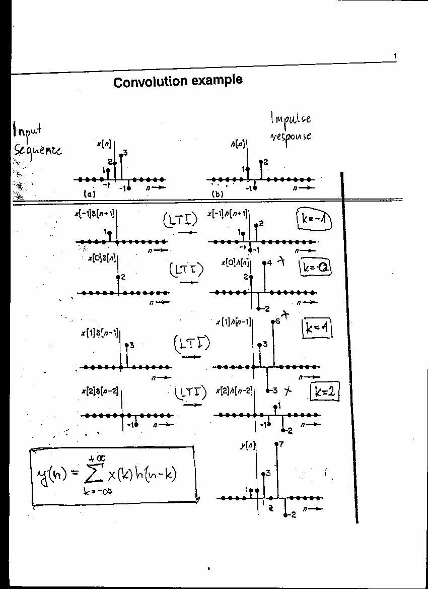
• Lecture 5 (22.11) LTI systems, convolution, z-transform (slides: newlect2.pdf, newlect7.pdf)
  Convolution example: conv_exampl.jpg
  HOMEWORK1 will be given (due 29.11)
• Lecture 6 (29.11) Z-transform and filter design
  Filters part I: newlect8.pdf
  Filters part II: newlect9.pdf
  Filters part III: newlect10.pdf Homework (hand-written on paper, worth up to 2 points) is due at the beginning of the lecture.
  
• Lecture 7(6.12): 14:15-15:00 one hour test I, 10pts worth: bring YOUR OWN notes (handwritten on paper or on printed lecture slides). No books, no photocopies of other person notes. Example test:test1_078a.pdf
  15:15-16:00 Filters lecture - continued
• Lecture 8 (13.12): FFT and filtering applied:
  Comb filter for decimation from "Filters part III:" newlect10.pdf
  Filtering (=convolution) with FFT from newlect5.pdf
  
• Lecture 9 (15.12): Digital signal processors: lect12_dsp.pdf(and OHP foils to be seen at the lecture)
  
• Lecture 10 (20.12): 2D signal processing lect13.pdf
  Homework:(homew2_2008plus.pdf) given today
• 26.12: Merry Christmas and Happy New Year
• Lecture 11 (3.1): 2D signal processing continued
  and signal processing for data compression
  Homework due today
• Lecture 12 (10.1): test II example test here; in problem 1a use M=6 or 4 (not 5, as it has to be even)
• Lecture 13 (17.1): Random DT signals
  Slides: lect_random.pdf;
• Lecture 14 (24.1):
  Advanced techniques lectadv.pdf
  + Review
• THE END OF SEMESTER

Exam tests 2007

There is no guarantee that the current test be identical ;-). It will be similar (the lecture was similar), but I might also put more focus on different subjects. The only base is the lecture content (live one, not only the published slides ....).

The main rule: exam covers the whole course content (sampled), including the T1(H1)+T2(H2) area and also the lectures after the H2.

Exam tests 2009 w/solution discussion

1. In both cases the signal was sampled correctly (f_s>2f)
   1. To calculate N₀ it was enough to count no. of samples in period (or divide f_s over f). Answer was 10(A) or 6(B). For N₀ samples in period, θ₀ was equal to 2π/N₀.
   2. K-size DFT will have K discrete samples over <-π, +π) (we include -π, and exclude +π , but due to periodicity of spectrum it is only a convention)
      for a cosine, only two samples are non-zero: at k such that θ_k=±θ_signal. Form the definition of θ_k you will see that this is for k=±4 (this is the result of taking K=4N₀).
   3. You may label frequency axis with k=-K/2,....-1,0,1,...K/2 or with its periodic equivalent K-K/2,....K-1,0,1,...K/2
      to label with θ just use the expression for θ_k.
2. 1. H(z)=Y(z)/X(z) is easily obtainable from the time equation. It was
      0.2(1+z^-1)/(1-0.8z^-1) [A]
      -0.2(1-z^-1)/(1+0.8z^-1) [B]
   2. Zeros are roots of numerator: -1 [A] or +1 [B]
      Poles are roots of denominator: +0.8 [A] or -0.8 [B]. They are inside unit circle, so the system is stable (but I didn't ask...)
   3. Example graph: - please find a_0, b_0, b_1 by yourselves. If you are smart, you may save one multiplication by 0.2 (this is left as exercise to you).
   4. For x(n)= shifted delta, (a limited energy signal) you may take the impulse response and shift it appropriately. To find h(n) it is easiest to split H(z) into two fractions: (shown for [A], for [B] change some signs)
      0.2(1/(1-0.8z^-1)+z^-1/(1-0.8z^-1))
      and lookup the inv.Z of 1/(1-0.8z^-1) in the table. The final result is a sum of two identical exponentials shifted by 1 in time. Then, you shift h(n) to proper position....
   5. For x(n) = 1-(-1)ⁿ (a periodic signal) we see a DC component and a periodic component exp(jπn) with frequency of π. We find numerical values of H(0)=(2 or 0) and H(π)= (0 or -2) by substituting exp(0) and exp(π) for z, and finally
      y(n)=H(0)-H(π)·(-1)ⁿ
3. The response was symmetrical around its midpoint (n= 2 or 4). Thus, it was a repsonse of a zero-phase filter delayed by 2 or 4.
   1. phase is linear φ=-(2 or 4)θ
      delay is constant and equal to (2 or 4)
   2. The response of filter is a rectangle modulated by exp(jπn). Thus, the characteristics is a sin(θL/2)/sin(θ), shifted to π. You may find the mainlobe width, you may plot exactly zeros of A(θ) etc.
4. Time resolution is proportional to time duration of window, frequency resolution - to mainlobe width (which is prop. to 1/K ....).
   Rectangular window has narrowest mainlobe possible, but high sidelobes; so it is good for resolving signals close in frequency, but without large difference in amplitudes.
   Any other window will have wider mainlobe (so poorer resolution in f).
5. 1. There was nonlinearity introcuced by product of two samples (linear is multiplication by a constant only).
      Saying "causal=yes because of BIBO" was not enough; "because FIR" was enough; if you call BIBO, you have to prove it by finding relation between bound of input and output.
   2. LP filter with passband of π/4 (see the "lecture 17").
   3. Many shorter is better: by averaging we reduce the variance of estimate. (variance is huuuuuge with single FFT)
   4. β (some call it α) controls the shape of window - effectively the sidelobes level (high β - low sidelobes).
   5. Inv FT is calculated by summation when the spectrum is discrete ([B], periodic signal) and by integration when the spectrum is continuous ([A], limited energy signal).
   6. 3 buses are for opcode, data1 (signal), data2 (coefficient).
      Any instruction with dual move uses all three, e.g MAC instruction needs 2 data, so it is nice that we can load data in the same cycle in 56002 it can be coded as:
      mac a,b x:(r0+),x0 y:(r4+),y0
   7. Trivial
   8. def: order of n^2, FFT: order of n log2(n)
   9. y(n) length is, maximally, (length of h(n))+(length of x(n))-1. K=M+N-1. Here, we were asked to find M knowing K and N. Answer is, as you may guess, M=K-(N-1)
   10. The clue is in word "maximally". It may happen that for certain signal (e.g in the stopband....) the y(n) is shorter.....

T1/T2 test examples

Try to solve the missing versions of tests.

Test1 ver.A problems
Test1 ver.B problems
Test1 ver.B solutions
Test1 ver.A solutions
Test2 (ver.A) and solutions
Test2 (ver.B) (do it yourself!)
Also, think first, act later.

• If you see a system - what type of system it is? LTI? What consequences arise from this?
• If you see a signal - is it limited energy? periodic?
• Which tool to use for LE? Which one for periodic? Which FT definition is appropriate?
• Is the plot you see in time or in frequency?
• Is the plot you have to sketch - in time or freq domain?
• Will the sketch requested be continuous or discrete? periodic? Will it have some symmetry? Is the function real-valued or complex? Maybe we are plotting abs()?
• maybe the function in freq can be expressed as "real times exp(j n0 theta)" because in time it is "symmetrical but shifted by n0"? How much is n0? (If in freq domain - shifted by θ0 - how much is this? )
• Signal is causal? Don't forget u(n) then.
• See -1? Try exp(j pi) instead. See exp(j pi)? Try (-1)....

Lab info: example lab exercises

Disclaimer:

Openly speaking, they are exercise sets current at the time of posting. I reserve the right to make some important modifications before the actual lab, to give different sets to different groups etc. (and I usually DO review the text before giving it....).

• Lab 0: Introduction, Matlab
• Lab 1: Signals, systems, frequency
  • Simple MATLAB usage: make a vector, plot x - y plot with proper data on axes, make a simple m-function.
  • DT signal as a sampled CT signal: plot sample values of a sin() with a frequency of 1 kHz, sampled with 10 kHz (etc). Put x-axis values as sample index, CT instant, ....
  • Normalized frequency concept (e.g. What is the θ value in the above example?)
  Lab exercises (and examples of entry test): nwlab1.pdf
• Lab 2: Spectral analysis
  • DFT properties, effect of limited observation time (windowing)
  • Spectrum of a rectangular impulse
  Lab exercises: nwlab2.pdf
• Lab 3: Instantaneous spectrum or STFT Lab exercises: lab03.pdf
  Example entry test:
  • Calculate the Fourier spectrum of a rectangular window with given length. Find the number of \{zero places|sidelobes\} and mainlobe width .
  • Calculate the DFT of a signal consisting of exactly 4 periods of a cosine, or 2 periods zero-padded to the length of 4 periods.
  • Calculate the STFT (inst. spectrum) of a u(t)cos(0.2π n) for a rectangular window of given length positioned at n=0, n=9, ....
  • We sample a signal with f_s=100 kHz and use boxcar window with length L=500 to calculate STFT. What is the approximate resolution of STFT in \{time|frequency\}?
• Lab 4: Filter design Lab exercises: lab4.pdf
  Example entry test below. Please DO these exercises.
  • Location of two poles and two zeros is given (here you may invent any decent location of zeros and poles). Calculate filter frequency characteristics.

    Hints:
    a) start from easy configurations, e.g. real zeros at +1 and -1, then zeros on the unit circle, double pole at z=0;
    b) First recall which root configurations are possible for a real-coefficient polynomial, then recall stability criterion for DT filter (poles inside unit circle) - don't use silly configurations

  • A filter structure is given. Find all its properties: h(n), H(z), poles/zeros, amplitude characteristics..... (for own exercises - use all the lecture examples first; read the newlect9.pdf for a reference)
  • A filter is characterized by H(z) (given). Find the output y(n) for x(n)=sin(θ₁n)+cos(θ₂n)+1 (or some other combination of different signals)
  • Explain step-by-step design process of FIR filter by windowing the ideal filter characteristics. Explain role of window (etc.).
• Lab 5: Signal processors Lab exercises: lab_emubox.pdf
  Example entry test problems:
  • Describe differences between Von Neumann and Harvard computer architectures.
  • Describe differences between a typical Digital Signal Processor and a typical {microcontroller|| general purpose processor - e.g. i386 || GPU}
  • Why does a DSP usually have {two or three memory buses || two address generators || bit-reversal addressing mode || hardware "for" loop implementation}? (Give an example of an instruction using this feature).
  • A system has been tested by applying a unit impulse at the input and recording the output sequence y[n]. Finally, an FFT has been computed from the y[n], and absolute value plotted. What do we see on the plot? Please describe assumptions that must be made!
• Lab 6: Image processing Lab exercises: lab_img_lx.pdf.

  Example entry test problems (see also last slide of lect13.pdf):

  • Calculate 2D-DFT of a simple (e.g. 4x4) image
  • Filter a trivial image (2D-delta, edge etc) with a given linear filter
  • Filter a trivial image (2D-delta, edge etc) plus some erroneous pixels with a median filter
  • Given some Fourier coefficients calculate the corresponding image (i.e. Inverse 2D-DFT)
  • Determine frequency content of a simple image (e.g: "Which frequency is represented by horizontal 1-1-0-0-1-1-0-0 stripes?")
  • Describe effects that may result from using {white-padding|black-padding|periodic padding|mirror padding} outside image borders when filtering with a linear filter.

Past things archive (Attic)