slides!

THIS PAGE IS NOT VALID NOW - PLEASE USE THE LINK BELOW

Shortcuts ABOUT What will all this be about? SLIDES Lecture slides SCHEDULE Dates of lectures/homeworks/tests/labs SCORES List of lab groups and scores LABS Info and examples of entry tests TESTS Test examples with hints for study

Current issues Office hours: Mon 16:30-17:00, room 454 Lecture start: 5th Oct (Thu), 08:15-10:00, room 121 Lab starts with an introductory meeting on 23rd Oct (Mon) 9:15, room CS202, Regular labs will be on odd ("N_blue"group) or even ("P_green" group) Mondays, 8:15-12:00 Lab group chooser will be started 5th Oct and closed on 13th Oct 10:00. Enter the link to chooser, then: assign grades to different variants (Put "5" if you really want to be in this subgroup, "4" for the second choice, .... down to "1" if it is really bad for you) leave some flexibility if possible (choose more than one acceptable variant), otherwise the assignment problem may be inconsistent. press the blue button "Zapisz" ("Save") -- I am sorry, the web system is still experimental and there is no English version. After the closing date of the chooser I will run the optimizer to assign subgroups, earlier I may make the decision on running/cancelling some subgroups, depending on the number of students registered. If you cannot access the chooser(e.g. you will not obtain your password before deadline) please mail me your choice of grades (5-very good, 4..,3..,2..,1-very bad) for the lab dates: [N-odd Mondays] [P-even Mondays] [F- even Fridays 10-14]. 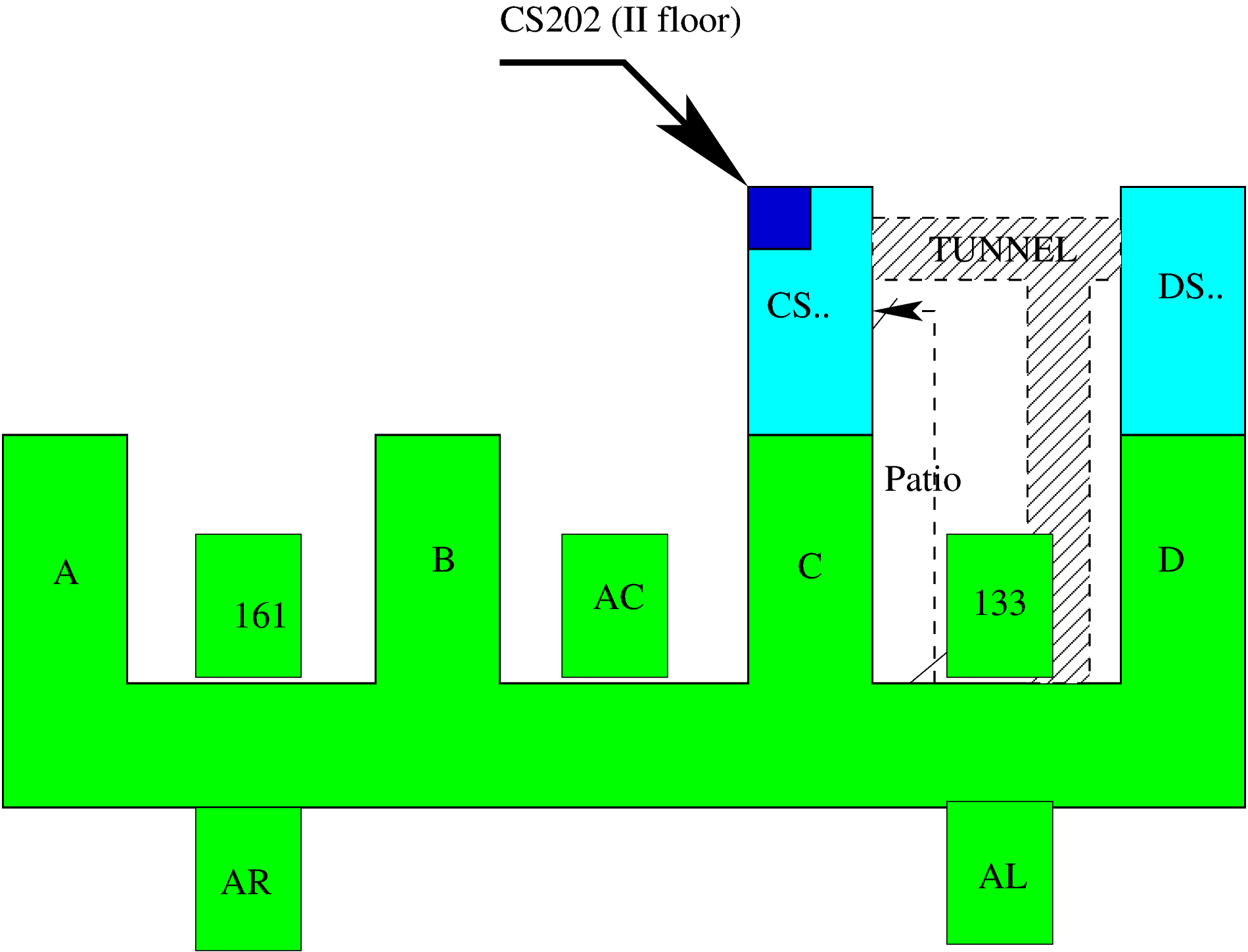Where is Lab CS202?

What to do after EDISP? If you are interested, choose elective courses: ETASP - (En) Techniques for Advanced Signal Processing EASP - (En) Adaptive Signal Processing or in Polish: TRA - Techniki Realizacji Algorytmów CPS PSYL - Przetwarzanie SYgnałów w Labview SRMP - Sygnały Radiolokacyjne i Metody ich Przetwarzania CCM - Czasowo-Częstotliwościowe Metody przetwarzania sygnałów APSG - Adaptacyjne Przetwarzanie SyGnałów

Home page of EDISP
(English) DIgital Signal Processing course
semester 2017z (autumn/winter of 2017/18 acad. year)

Schedule

There are lab exercises, 4 hours every second week, room CS202 (new wing C).

Labs will be on Mondays, 8-12 (N and P weeks) or Fridays 10-14 (P weeks; Fri is only available if the group is LARGE) , in subgroups of not more than 12 students.

For the introductory lab (lab0) we ALL met on Mon, 23rd Oct , 9:15 in room CS202.
Next lab (lab1) will be

• Oct 30th (8:15-12) for P (Parity even) subgroup
• Nov 6th (8:15-12) for N (Non-parity = parity odd) subgroup,

• In some weeks the weekdays are swapped to equalize the semester,
• In some semesters the notion of "odd" (N) and "even" (P) in that calendar may be not as straightforward as taught within a basic algebra course.

Books

Book base

A. V. Oppenheim, R. W. Schafer, Discrete-Time Signal Processing, Prentice-Hall 1989 (or II ed, 1999; also acceptable previous editions entitled Digital Signal Processing).

Other books

• Steven W. Smith, The Scientist and Engineer's Guide to Digital Signal Processing - it is a free textbook covering some of the subjects, to be found here: http://www.dspguide.com/pdfbook.htm
  The book is slightly superficial, but it can be valuable - at least as a quick reference.
• Edmund Lai, Practical Digital Signal Processing for Engineers and Technicians, Newnes (Elsevier), 2003
  seems also a simple but thoroughly written book.
• Vinay K. Ingle, John G. Proakis, Digital Signal Processing using MATLAB, Thomson 2007, Bookware Companion series
  

Supplementary books I found in our faculty library:

Additional books available in Poland:

• R.G. Lyons, Wprowadzenie do cyfrowego przetwarzania sygnałów (WKiŁ 1999)
• Craig Marven, Gilian Ewers, Zarys cyfrowego przetwarzania sygnałów, WKiŁ 1999 (simple, slightly too easy) [en: A simple approach to digital signal processing, Wiley & Sons, 1996]
• Tomasz P. Zieliński, Od teorii do cyfrowego przetwarzania sygnałów, WKiŁ 2002 (and next edition with slightly modified title)

Please remember:

• there are notation differences between lecture and "dspguide"
• The official book is Oppenheim & Schafer (though notation is sometimes different too)
• no book is obligatory as it is hard to get O&S, and other books do not cover the subject fully.

Probably the best choice is to buy a used copy of O&S. It'll serve you for years, if you are interested in DSP. And it contains a lot of PROBLEMS to solve and learn!

Ingle/Proakis is also a good book (and you may be able to buy a new or almost new copy).

If you know LANG=PL_pl - you may prefer to buy/borrow a laboratory scriptbook for CYPS, which is in Polish language (Cyfrowe Przetwarzanie Sygnałów, red. A Wojtkiewicz, Wydawnictwa PW).
 

Supplementary material

Course aims

A student who successfully completes the course will:

• know the mathematical fundamentals of discrete-time (DT) signal processing: DT signals, normalized frequency notion, DT systems, LTI assumption, impulse response, stability of a system
• understand the DT Fourier transforms and know how to apply them to simple DT signal analysis
• know basic window types and their usage for FT and STFT
• understand the description of a DT system with a graph, difference equation, transfer function, impulse response, frequency response
• be able to apply Z-transform in analysis of a simple DT system
• understand filtering operation and the process of DT filter design; be able to use computer tools for this task
• know the basic attributes of a Digital Signal Processor (differences w.r.t. general purpose processor, ways of speeding up the calculations, fundamentals of block diagram and programming)
• understand 2D signal processing basics: 2D convolution/filtering, 2D Fourier analysis
• be able to use a numerical computer tool (Matlab, Octave or similar) for simulating, analyzing and processing of DT signals

Lecture slides

• Lecture 1 slides: (intro, signals) newerlect1.pdf
• Lecture 2 slides: (sampling, frequency) newerlect1.pdf (from slide 12)
  and
  newerlect2.pdf
• Lecture 3 slides (frequency, FT od periodic signals, DFT): (idea of a transform, FT - Fourier Transform of L2 signals) newerlect2.pdf
• Lecture 4 slides - DFT: newerlect2.pdf (continued)
  and windowing \& FFT newerlect3.pdf
• Lecture 5:
  FFT - newerlect3.pdf
  Short-Time Fourier Transform (STFT, instantaneous spectrum): newlect6.pdf

• Lecture 6
  FFT - Fast Fourier Transform
  STFT - Short-Time Fourier Transform (STFT, instantaneous spectrum): newlect6.pdf
  
  LTI systems, convolution, z-transform
  lect_lti_z.pdf
  
• Lecture 7 z-transform
  lect_lti_z.pdf continued
  HOMEWORK1 will be given (due 20.04)
• 13 Apr - holidays start...
• Lecture 8 (20 Apr 2017) filters, filter design:
  lect_filt.pdf
  Filters - advanced design, tips, tricks lect_filtadv.pdf
  HOMEWORK1 (due in the middle break)
• Lecture 9 (27 Apr 2017): Test I
  
  • One hour test I, 10pts worth: bring YOUR OWN notes (handwritten on paper or on printed lecture slides). No books, no photocopies of other person notes.
    The test will cover the subjects which were in the Homework1 i.e. up to (and including) LTI systems and comvolution/impulse response.
    Example test:test1_078a.pdf
    More examples w/solution: down in the page
  • Filters lecture - continued.
    
• 4 May 2017: NO LECTURE
• Lecture 10 (11 May 2017): Filters lecture - continued.
  
• Lecture 11 (18 May 2017): Implementing DSP lect_implem.pdf
  Homework2 start - please download from homew2_2008plus.pdf.
• Lecture 12 (25 May 2017):
  2D signals: newlect13_2d.pdf
  and
  signal processing for data compression
  Homework 2 due today
• Lecture 14 (1 Jun 2017):
  2D signals continued
  signal processing for data compression
  Advanced techniques;
  
• Lecture 13 (8 Jun 2017):
  test II
  example test here; in problem 1a use M=6 or 4 (not 5, as it has to be even)
  More test examples in test examples section.
• THE END OF SEMESTER

Examples of tests

Exam tests 2007

There is no guarantee that the current test be identical ;-). It will be similar (the lecture was similar), but I might also put more focus on different subjects. The only base is the lecture content (live one, not only the published slides ....).

The main rule: exam covers the whole course content (sampled), including the T1(H1)+T2(H2) area and also the lectures after the H2.

Exam tests 2009 w/solution discussion

1. In both cases the signal was sampled correctly (f_s>2f)
   1. To calculate N₀ it was enough to count no. of samples in period (or divide f_s over f). Answer was 10(A) or 6(B). For N₀ samples in period, θ₀ was equal to 2π/N₀.
   2. K-size DFT will have K discrete samples over <-π, +π) (we include -π, and exclude +π , but due to periodicity of spectrum it is only a convention)
      for a cosine, only two samples are non-zero: at k such that θ_k=±θ_signal. Form the definition of θ_k you will see that this is for k=±4 (this is the result of taking K=4N₀).
   3. You may label frequency axis with k=-K/2,....-1,0,1,...K/2 or with its periodic equivalent K-K/2,....K-1,0,1,...K/2
      to label with θ just use the expression for θ_k.
2. 1. H(z)=Y(z)/X(z) is easily obtainable from the time equation. It was
      -0.2(1+z^-1)/(1-0.8z^-1) [A]
      0.2(1-z^-1)/(1+0.8z^-1) [B]
   2. Zeros are roots of numerator: -1 [A] or +1 [B]
      Poles are roots of denominator: +0.8 [A] or -0.8 [B]. They are inside unit circle, so the system is stable (but I didn't ask...)
   3. Example graph: - please find a_0, b_0, b_1 by yourselves. If you are smart, you may save one multiplication by 0.2 (this is left as exercise to you).
   4. For x(n)= shifted delta, (a limited energy signal) you may take the impulse response and shift it appropriately. To find h(n) it is easiest to split H(z) into two fractions: (shown for [A], for [B] change some signs)
      0.2(1/(1-0.8z^-1)+z^-1/(1-0.8z^-1))
      and lookup the inv.Z of 1/(1-0.8z^-1) in the table. The final result is a sum of two identical exponentials shifted by 1 in time. Then, you shift h(n) to proper position....
   5. For x(n) = 1-(-1)ⁿ (a periodic signal) we see a DC component and a periodic component exp(jπn) with frequency of π. We find numerical values of H(0)=(2 or 0) and H(π)= (0 or -2) by substituting exp(0) and exp(π) for z, and finally
      y(n)=H(0)-H(π)·(-1)ⁿ
3. The response was symmetrical around its midpoint (n= 2 or 4). Thus, it was a repsonse of a zero-phase filter delayed by 2 or 4.
   1. phase is linear φ=-(2 or 4)θ
      delay is constant and equal to (2 or 4)
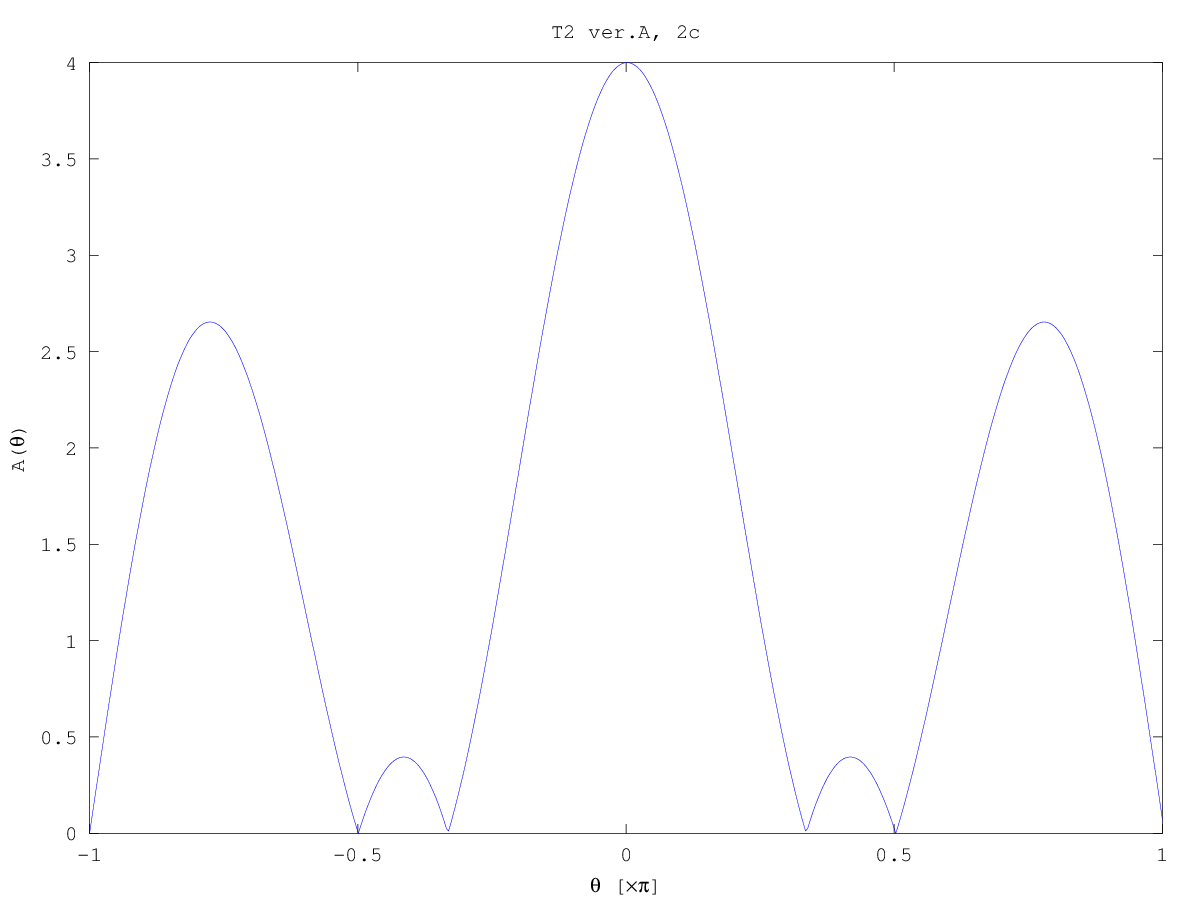
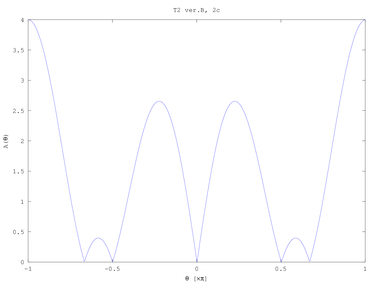
   2. The response of filter is a rectangle modulated by exp(jπn). Thus, the characteristics is a sin(θL/2)/sin(θ), shifted to π. You may find the mainlobe width, you may plot exactly zeros of A(θ) etc.
4. Time resolution is proportional to time duration of window, frequency resolution - to mainlobe width (which is prop. to 1/K ....).
   Rectangular window has narrowest mainlobe possible, but high sidelobes; so it is good for resolving signals close in frequency, but without large difference in amplitudes.
   Any other window will have wider mainlobe (so poorer resolution in f).
5. 1. There was nonlinearity introcuced by product of two samples (linear is multiplication by a constant only).
      Saying "stable=yes because of BIBO" was not enough; "because FIR" was enough; if you call BIBO, you have to prove it by finding relation between bound of input B_x and output B_y.
   2. LP filter with passband of π/4 (see the "lecture 17").
   3. Many shorter is better: by averaging we reduce the variance of estimate. (variance is huuuuuge with single FFT)
   4. β (some call it α) controls the shape of window - effectively the sidelobes level (high β - low sidelobes). Is high β better? yes, if you are concerned with sidelobe level; but remember that you pay with wider mainlobe (There Ain't No Such Thing As A Free Lunch)
   5. Inv FT is calculated by summation when the spectrum is discrete ([B], periodic signal) and by integration when the spectrum is continuous ([A], limited energy signal).
   6. 3 buses are for opcode, data1 (signal), data2 (coefficient).
      Any instruction with dual move uses all three, e.g MAC instruction needs 2 data, so it is nice that we can load data in the same cycle in 56002 it can be coded as:
      mac a,b x:(r0+),x0 y:(r4+),y0
   7. Trivial
   8. def: order of n^2, FFT: order of n log2(n)
   9. y(n) length is, maximally, (length of h(n))+(length of x(n))-1. K=M+N-1. Here, we were asked to find M knowing K and N. Answer is, as you may guess, M=K-(N-1)
   10. The clue is in word "maximally". It may happen that for certain signal (e.g in the stopband....) the y(n) is shorter.....

Exam test 2012/13

T1/T2 test examples

Try to solve the missing versions of tests.

Test1 2010/11 ver.A problems
Test1 2010/11 ver.B problems
Test1 ver.B solutions
Test1 ver.A solutions
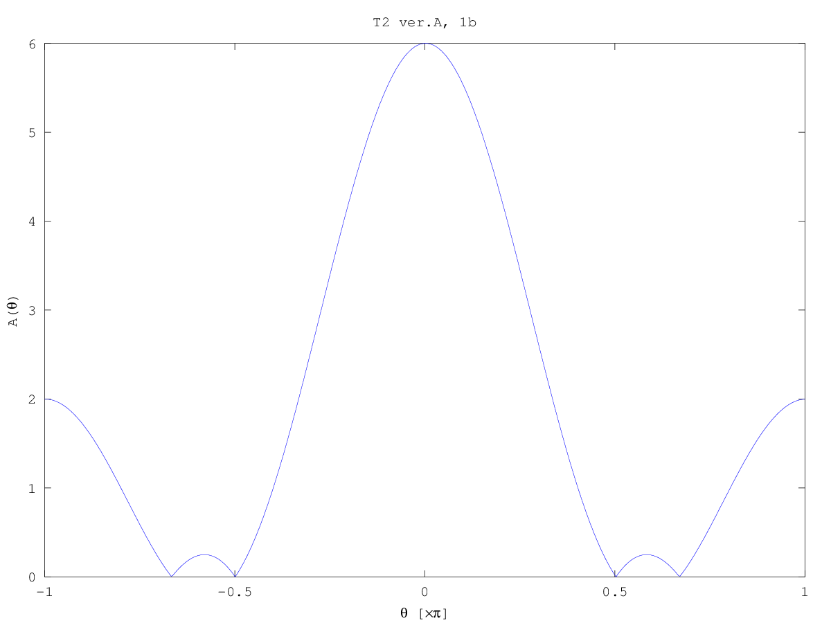
Test2 2016L ver A. solved
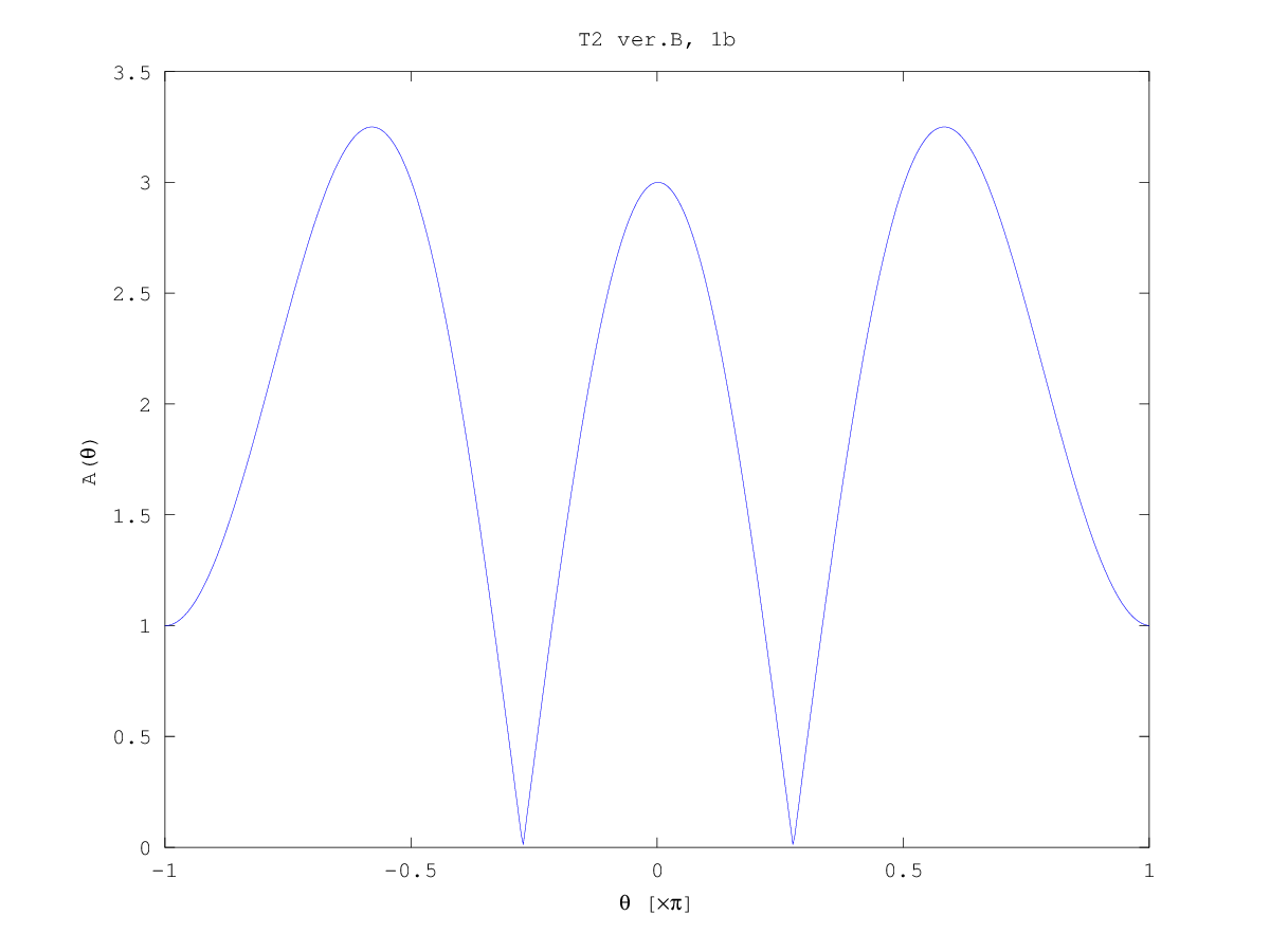
Test2 2016L ver B. (do it yourself)
Test2 (ver.A) and solutions
Test2 (ver.B) (do it yourself!)
Also, think first, act later.

• If you see a system - what type of system it is? LTI? What consequences arise from this?
• If you see a signal - is it limited energy? periodic?
• Which tool to use for LE? Which one for periodic? Which FT definition is appropriate?
• Is the plot you see in time or in frequency?
• Is the plot you have to sketch - in time or freq domain?
• Will the sketch requested be continuous or discrete? periodic? Will it have some symmetry? Is the function real-valued or complex? Maybe we are plotting abs()?
• maybe the function in freq can be expressed as "real times exp(j n0 theta)" because in time it is "symmetrical but shifted by n0"? How much is n0? (If in freq domain - shifted by θ0 - how much is this? )
• Signal is causal? Don't forget u(n) then.
• See -1? Try exp(j pi) instead. See exp(j pi)? Try (-1)....

Test1 2013/14 ver.A problems

• Max score was 13, I assume 10 is OK, and +3 is a bonus.
• Typical errors as I commented by email on your homework still show up.
• Hints:
  1. Impulse response is useful if system is LTI (Linear AND Time-Invariant -- you must verify both!)
     Stability is verified by finding M such that By=M Bx; one way to find M is to calculate ∑ |h(n)|. Remember that h(n) → 0 is NOT enough (look here for an example)
  2. Remember that fn or N are UNITLESS (don't use units like Hertz or seconds) -- they are ratios of f/fs or just number of samples
     Common error -- forgetting that there is N0 and N, and N must be an integer (N=19 [A] or 9 [B])
  3. FFT complexity calculation was simple (answer: [A] 48 ms, [B] 2 ms)
  4. DTFT was either 2cosθ or -2jsinθ. The task was to plot AMPLITUDE |X(θ)|, then to recall that DFT-8 will be just 8 samples of X(θ)
  5. Formula N+L-1 is good as a maximum length of convolution if we don't know exactly signals. In this case h(n) was a short rectangular pulse, x(n) -- two well-separated deltas, so in the output we got just two copies of h(n). ([A]:10, [B]:14, however I gave 1/2 score for correct application of L+N-1)
     Put this code in Octave or Matlab:
     

     	    x=zeros(1,100);
     	    n=[1:100]-10;
     	    x(n==0)=1;
     	    x(n==40)=1;
     	    figure(1);
     	    stem(n,x); title('x(n)');axis([-20 100 0 1.2]);
     	    h=ones(1,5);
     	    figure(2);
     	    stem(0:4,h); title('h(n)');axis([-20 100 0 1.2]);
     	    figure(3)
     	    y=conv(x,h);
     	    stem([1:length(y)]-10,conv(x,h));axis([-20 100 0 1.2]);
     	  

  6. xs(n) was a SUM of x(n) with manipulated x(n):
     1. shifted by N → X(k)⋅ exp(-j N θ_k) ; happily this factor is always =1;
     2. inverted in time → X(-k) (or X*(k) for real signals)
     Some students applied linearity idea in the argument of X(k) (WRONG!!!! Do it only on X, not on k)

Test 2 (2013/14) solutions sketch
Computer plots:

Test 1 (2016z) solved

Lab info: example lab exercises

• Ms. Anna Kurowska
  email:a.kurowska(*)elka.pw.edu.pl
  room 447
• Mr. Maciej Wielgo
  email:m.wielgo(*)elka.pw.edu.pl
  room 447
• Prof. Krzysztof Kulpa
  email:kkulpa(*)elka.pw.edu.pl
  room 453
• Dr. Jacek Misiurewicz
  email:jmisiure(*)elka.pw.edu.pl
  room 454

Disclaimer:

Openly speaking, they are exercise sets current at the time of posting. I reserve the right to make some important modifications before the actual lab, to give different sets to different groups etc. (and I usually DO review the text before giving it....).

Lab exercises:

• Lab 0
  Introduction, Matlab (and no entry test).
  There is no written instruction for lab0.
• Lab 1
  Signals, systems, frequency
  • Simple MATLAB usage: make a vector, plot x - y plot with proper data on axes, make a simple m-function.
  • DT signal as a sampled CT signal: plot sample values of a sin() with a frequency of 1 kHz, sampled with 10 kHz (etc). Put x-axis values as sample index, CT instant, ....
  • Normalized frequency concept (e.g. What is the θ value in the above example?)

  Prepare to the lab1

  Take a look at lab exercises (and examples of entry test) and:
  • try to do the example entry test
  • go carefully through lab exercises and visit http://www.mathworks.com/help/matlab/ to find help/explanations for commands that are used in the instructions (e.g. cumsum(), ":" operator for array subscripting [search Mathworks for "colon"], zeros(), ones(), stem() )
  Optional: visit http://www.gnu.org/software/octave/ and install Octave - then you will be able to do the simulation experiments at home (100% legally); you may also learn commands using e.g. "help colon" from the octave prompt instead of mathworks site. [note: "getdata()" and some special scripts will not work under Octave; "getdata()" works only for the A/D card in lab, local scripts are present only in lab computers].
  
• Lab 2
  Spectral analysis
  • DFT properties, effect of limited observation time (windowing)
  • Spectrum of a rectangular impulse
  For entry test examples see the lab instruction booklet.
• lab3
  Instantaneous spectrum or STFT
  Example entry test:
  • Calculate (and sketch) the magnitude Fourier spectrum of a rectangular window with given length L. Find the number of \{zeroes|sidelobes\} and mainlobe width .
  • Sketch the DFT of a signal consisting of exactly 4 periods of a cosine, (or: 2 periods of cosine, zero-padded to the length of 4 periods).
  • Calculate the STFT (inst. spectrum) of a u(n)cos(0.2π n) for a rectangular window of given length positioned at n=0, n=9, .... (choose length>10)
  • We sample a signal with f_s=100 kHz and use boxcar window with length L=500 to calculate STFT. What is the approximate resolution of STFT in \{time|frequency\}? (a variant: we want to resolve two signals spaced by 1 kHz -- what length do we need?)
• Lab4
  Filter design
  Example entry test below. Please DO these exercises.
  • Location of two poles and two zeros is given (here you may invent any decent location of zeros and poles). Calculate filter frequency response (magnitude response).

    Hints:
    

    • start from easy configurations, e.g.
      1. real zeros at +1 and -1,
      2. pair of zeros somewhere on the unit circle, double pole at z=0;
      3. pair of poles at a given angle and radius a bit smaller than unit, double zero at z=0
    • (this is not from EDISP lecture but from MATH lecture!) First recall which root configurations are possible for a real-coefficient polynomial, then recall stability criterion for DT filter (poles inside unit circle) - don't use silly configurations
  • A filter structure is given. Find all its properties: h(n), H(z), poles/zeros, magnitude response..... (for own exercises - use all the lecture examples first; read the lect_lti_z.pdf and lect_filt.pdf for a reference)
  • A filter is characterized by H(z) (given). Find the output y(n) for x(n)=sin(θ₁n)+cos(θ₂n)+1 (or some other combination of different signals)
    Hints:
    • recall that convolution with a given h(n) is a linear operator -- decompose x(n) into separate easy components
    • Substitute exp(jθ) into z
    • find amplitudes for interesting θ values
    • find phases for these θ values
  • Explain, step-by-step, the design process of FIR filter by windowing the ideal filter characteristics. Explain role of window (etc.).
• Lab 5
  Implementing DSP
  Some example entry test questions are in the instruction PDF.
• Lab 6
  Image processing

  Example entry test problems are in the lab script (above) and also here:

  • Calculate 2D-DFT of a simple (e.g. 4x4) image
  • Filter a trivial image (2D-delta, edge etc) with a given linear filter
  • Filter a trivial image (2D-delta, edge etc) plus some erroneous pixels with a median filter
  • Given some Fourier coefficients calculate the corresponding image (i.e. Inverse 2D-DFT)
  • Determine frequency content of a simple image (e.g: "Which frequency is represented by horizontal 1-1-0-0-1-1-0-0 stripes?")
  • Describe effects that may result from using {white-padding|black-padding|periodic padding|mirror padding} outside image borders when filtering with a linear filter.

Past things archive (Attic)